The Ideal Flow Machine Matlab program provides an environment to explore the structure and form of two-dimensional potential flows. It was used to generate a number of figures in section 2.7 of the book and is a useful instructional tool for potential flow theory from elementary flows to conformal mapping. Download here.

Instructions

The Ideal Flow Machine

The Ideal Flow Machine is designed for undergraduate and graduate students who wish to understand elementary ideal flow in two dimensions. The term ‘Ideal flow’ describes the way in which a fluid (liquid or gas) moves when the effects of compressibility and viscosity are negligible. Ideal flow is often the first type of fluid motion that student engineers and scientists study, because it is the simplest. Large parts of the flows past ships, submarines, cars and light aircraft are closely ideal.

This applet is designed to give students an environment where they may experiment with and visualize elementary two-dimensional ideal flows and thus better understand them. The following description assumes the reader has had some theoretical introduction to this subject. Ideal fluid flows are solutions to Laplace’s equation. This differential equation is linear, which means that adding together (superposing) any number of ideal flows produces a new ideal flow. One approach to finding the solution to complex flow problems – termed superposition – is therefore to begin with very simple ideal flows, that are easily understood and described, and then to add them together to produce the complex flow patterns desired. This is exactly the process modelled in The Ideal Flow Machine.

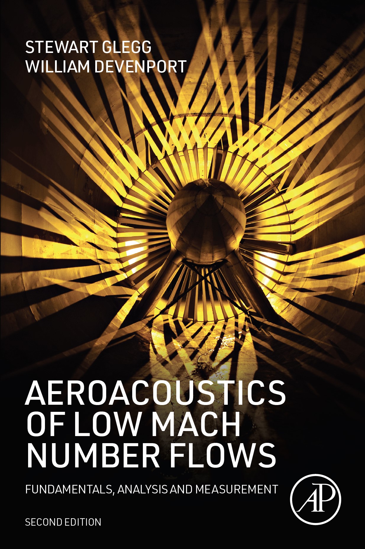
When you run the function ifm.m in Matlab, you will first see a window like that shown below –

The window shows a grid. Above the grid is a dropdown menu with the selections; ‘Freestream’, ‘Source’, ‘Vortex’, ‘Doublet’, ‘Source panel’, ‘Vortex panel’, ‘Circle’, ‘Circle with K.c.’, ‘Draw Streamline+’, ‘Draw Streamline-‘, ‘Draw Potential+’ and ‘Draw Potential-‘. Adjacent to that is an editable text field (for entering the strength, angle or functional form of a flow), an ‘Undo’ button (to undo the last change you made), non-editable fields ‘X’ and ‘Y’ that show the position of the mouse on the grid and, at far right, a free stream indicator (that initially shows no free stream).

In short, what you do is select the type of flow you want to add, type in the strength/angle or functional form, as appropriate, and then click the mouse on the grid at the point where you want that flow to appear. You may add any number of sources, vortices doublets, source sheets or vortex sheets. Then you select one of the ‘Draw Streamline’ or ‘Draw Potential’ options and the computer will draw streamlines or equipotentials starting wherever you click your mouse on the grid. The whole thing is supposed to be a little like a real water tunnel, in which you set up your flow and then visualize the streamlines by adding dye at specific points (i.e. a Hele Shaw table, for those who remember).

When adding a freestream (usually a uniform flow in a given direction) both the strength and angle in degrees may be specified in the editable text field (e.g. ‘1,10’), but as long as you click somewhere in the grid, the position is irrelevant (this flow is the same everywhere). A function describing a non-uniform freestream may also be specified by typing the function into the text box in terms of the complex variable ‘z’ (e.g. ‘z^2+2*z’). The direction of a uniform freestream is indicated by an arrow that appears in graphic top right. If you entered a function this arrow will change to a script ‘f’ symbol to indicate that. It only makes sense to have one freestream. If you add a second it will simply overwrite the first.

When adding a source (a flow out from a point, or into a point when the strength is negative) specify a single numeric value for its strength. The source is indicated by a blue ‘+’ .

When adding a vortex (flow circulating around a point) again specify a single numeric value for its strength. The vortex is indicated by a red circle with a dot at the center.

Each doublet (flow out of one side of a point and back into the other) is indicated by a black star. You wll need to specify a numeric strength and angle (in degrees) for this flow (e.g. ‘1,45’).

A source panel is a source stretched out into a line. Likewise for a vortex panel. These are indicated by blue and red lines respectively. To add a sheet you click on the place where you want the sheet to start and then drag the mouse to draw out the sheet. Before drawing enter one or two numeric values in the text box separated by a comma to specify either a constant or linearly varying strength, respectively.

Selecting ‘Draw Streamline+’, ‘Draw Streamline-‘, ‘Draw Potential+’ or ‘Draw Potential-‘ allows you to visualize the flow you created. Draw streamline+ draws streamlines along the flow direction. Draw streamline- draws them against the flow direction. Draw potential+ and Draw potential- similarly allow you to visualize the potential lines of a flow which, by definition, are perpendicular to the streamlines. When one of these selections is chosen, clicking the mouse once on the plot will draw a streamline or potential line starting at that point. Dragging the mouse to define a line across the plot will draw a set of streamlines or potential lines starting on that line. Note that when a streamline/potential line comes to a point where the flow is stopped (a stagnation point) it will stop (just as dye would if injected into a flow). If it goes through the exact point where singularity (source, vortex, doublet, sheet ends) is located it will also stop, since the flow is undefined there. Streamlines or potential lines are colored according to the local flow velocity using the color scale at the bottom left of the window.

If you are unfamiliar with the types of flow described here, add one of them (and nothing else) and then draw some streamlines to see what it looks like.

The choice-menu selections ‘Circle’ and ‘Circle with K.c.’ allow you to apply the Milne Thompson Circle Theorem to a flow. This theorem allows you to create a circular streamline in any flow, simply by manipulating the function that describes that flow. To use this feature, first put together a flow in which you want to create a circular streamline using the tools described above. Then select ‘Circle’. Click the mouse at a point within the grid where you want your circular streamline to be centered and then drag the mouse to select the radius. Visualize the results using a ‘Draw Streamline’ option. Note that you can only add one circle at a time (adding a second simply overwrites the first). The option ‘Circle with K.c.’ functions in the same way, except that it allows you, additionally to specify the point at which the flow detaches from (or attaches to) the circle (i.e. you get to specify a Kutta Condition). This point is specified by the location where you release the mouse after dragging it to create the circle. A good way to test both of these options is to try them on a uniform flow. Note, however, that they will work on any flow, however complex.

On the bottom left of the window the limits of the color scale used for indicating velocity when plotting streamlines and potential lines can be adjusted. Clicking on the scale itself will change the color map. The buttons marked ‘+’ and ‘-‘ zoom the grid in or out. Note that the regular Matlab window ‘hand’ tool can be used to drag the position of the grid as desired.

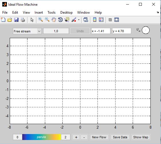
There are three buttons at the bottom of the frame. ‘New Flow’ allows you to erase whatever elementary flows (and circle) you have created so that you can start with a clean slate. ‘Show Data’ saves a .mat file containing all the information about the flow and streamlines you created. The third button ‘Show Map’ enables you to modify the flow you have generated using conformal mapping, as discussed below.

The Mapping Window

Pressing the ‘Show Map’ button in the Ideal Flow Machine window brings up a second window in which you can explore conformal mapping techniques. Conformal mapping is an advanced topic, usually taught to graduate students.

Conformal mapping follows from the description of two-dimensional ideal flows in terms of complex numbers . This description is a very natural one. Suppose you use a complex number to represent positions in two dimensions, e.g. z = x + iy. Then, by definition, any analytic (differentiable) function of the complex variable ‘z’ is a solution to Laplace’s equation – the governing equation of ideal flow. We can therefore describe any 2D flow as a function of z.

The problem with this result is that one does not know a priori which function of z will produced the specific flow of interest. We have already met one approach to this problem – the method of superposition – where we add very simple ideal flows together to produce the complex flow patterns desired. The description of ideal flows in terms of complex numbers, however, allows for an additional route – the distortion of one flow into another by conformal mapping. Conformal mapping involves the transformation of the complex coordinate ‘z’ into a different coordinate, say, z1 via a function, i.e. z1=z1(z). This process also transforms the flow, described say by a function F(z), to a new flow F1(z1) = F(z(z1)). As long as the derivative of the mapping function z1=z1(z) is not zero, then it turns out that the mapped flow is a solution to Laplace’s equation and is thus valid. At points where the derivative is zero, termed critical points, the mapped flow is not valid. Paradoxically, these points turn out to be particularly useful when trying to create sharp corners in a flow, such as at the trailing edge of the airfoil.

This process of mapping a flow in the complex plane is what is illustrated by the mapping window. When you press the ‘Show Map’ button, a window like that shown below will appear –

The mapping window is arranged similarly to the Ideal Flow Machine window. Top left is a drop down menu with the choices ‘z’, ‘az^b’, ‘a(z+b/z)’, ‘a ln(z) – ib’, ‘a(exp(bz) + bz), ‘(z-a)/(az-1) + b’, and ‘Custom’. These control the mapping function. The default mapping function is just z (i.e. duplication). If you click ‘Apply Map’ in this condition, a copy of any streamline/potential line maps you generated in the Ideal Flow Machine window will appear (after a short computational delay). To change the mapping function use the dropdown menu to select the functional form, the ‘a’ and ‘b’ constants are entered as numerical values (separated by a comma) in the text box to the right of the dropdown. (Note that, depending on the functional form you choose there are a few values of ‘a’ and ‘b’ that lead to meaningless results. If you happen to choose these an error window will warn you.) For a custom mapping enter the mapping function in terms of the variable z and numerical constants into the text box, e.g. “sin(z)+3i”. Once the mapping has been entered click ‘Apply Map’ and the streamline and/or potential line pattern will be drawn accordingly. If you add more streamlines to, or otherwise change, your original flow the corresponding streamlines will be added to the mapping window.

One important effect to watch out for is branching. A single flow in the z-plane can map to several different, and overlapping, flows in the mapped plane (branches). This is entirely correct, but it can be very ugly when you get overlapping streamline patterns. The number of possible branches can be trimmed somewhat by restricting the range of angles in the z-plane to -pi to pi (as is done here). There are still plenty of combinations of mapping and flow that will produced multiple branches though, so if you just want to see one branch be careful where you click the mouse. A useful tool for combining branches that are not consistent with default -pi to pi range is the ‘Hold’ button. This prevents any streamline pattern you have drawn from being erased when you change the mapping function. Then you can change the mapping function to explicitly bring up a different branch, and combine the results of those branches in different flow regions to create a single flow.

The mapping window also has labels that show the x and y position of the mouse in the mapped plane and an editable color scale that as before relates the color of the streamlines/potential lines to the velocity of the flow.

Please email if you have comments or suggestions (or you discover bugs).

William Devenport